Binary Plots

import poisson_approval as pa
from fractions import Fraction

XyyToProfile

In Poisson Approval, we call binary plot a graphical study of some profiles that are based on two rankings, denoted left_ranking and right_ranking, in various proportions, and where the utility of the voters for their second candidate also varies. To achieve this, we need an XyyToProfile object that will generate the profiles:

xyy_to_profile = pa.XyyToProfile(
    pa.ProfileNoisyDiscrete,
    left_ranking='abc',
    right_ranking='cba',
    d_type_fixed_share={('bac', 0.1, 0.01): Fraction(1, 12),
                        ('bac', 0.9, 0.01): Fraction(1, 12)},
    noise=0.01
)

The above syntax defines a function xyy_to_profile that maps a tuple \((x, y1, y2)\) to a profile defined as:

• The class of profile is ProfileNoisyDiscrete,

• A fixed share 1/12 of voters are of type \((bac, 0.1, 0.01)\), and a fixed share 1/12 of voters are of type \((bac, 0.9, 0.01)\),

• The other voters, i.e. a share 5/6, are distributed between left_ranking and right_ranking, in respective proportions \(1 - x\) and \(x\).

• The voters with preference order left_ranking have a utility \(y1\) for their second candidate,

• The voters with preference order right_ranking have a utility \(y2\) for their second candidate.

For example:

xyy_to_profile(x=Fraction(1, 5), y1=0.42, y2=0.51)

<abc 0.42 ± 0.01: 2/3, bac 0.1 ± 0.01: 1/12, bac 0.9 ± 0.01: 1/12, cba 0.51 ± 0.01: 1/6> (Condorcet winner: a)

Scale

All the plots require two resolution parameters called xscale and yscale. For example, if xscale = yscale = 10, then the x-axis and the y-axis are divided into cells of diameter 1/10 and the value of the plotted function is computed at the center of each cell. In this tutorial, we define global parameters XSCALE and YSCALE and we will use them for all the plots.

XSCALE = 10
YSCALE = 10

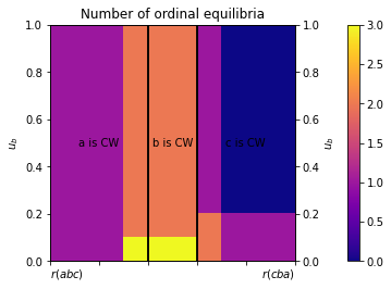
Number of Equilibria

By default, the function binary_plot_n_equilibria computes the ordinal equilibria, i.e. those where all voters having the same ranking cast the same ballot:

pa.binary_plot_n_equilibria(
    xyy_to_profile,
    xscale=XSCALE, yscale=YSCALE,
    title='Number of ordinal equilibria')

(<Figure size 414x288 with 3 Axes>,
 <poisson_approval.meta_analysis.binary_plots.BinaryAxesSubplotPoisson at 0x1e2d1f355f8>)

Using the option meth, you can investigate other kinds of equilibria:

pa.binary_plot_n_equilibria(
    xyy_to_profile,
    xscale=XSCALE, yscale=YSCALE,
    title='Number of group equilibria',
    meth='analyzed_strategies_group')

(<Figure size 414x288 with 3 Axes>,
 <poisson_approval.meta_analysis.binary_plots.BinaryAxesSubplotPoisson at 0x1e2d1d4ddd8>)

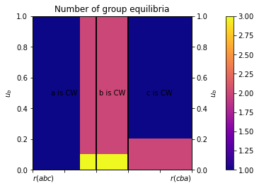
Depending on the class of profile, the possible values of the option meth may be:

• 'analyzed_strategies_ordinal' (the default),

• 'analyzed_strategies_group',

• 'analyzed_strategies_pure' (for ProfileDiscrete only).

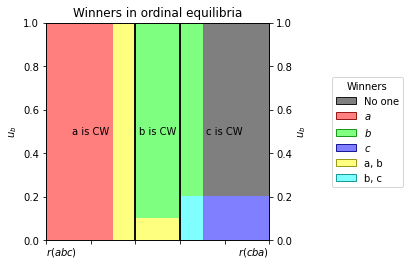
Winners at Equilibrium

The function binary_plot_n_equilibria works similarly:

pa.binary_plot_winners_at_equilibrium(
    xyy_to_profile,
    xscale=XSCALE, yscale=YSCALE,
    title='Winners in ordinal equilibria')

(<Figure size 288x288 with 2 Axes>,
 <poisson_approval.meta_analysis.binary_plots.BinaryAxesSubplotPoisson at 0x1e2d2346a20>)

pa.binary_plot_winners_at_equilibrium(
    xyy_to_profile,
    xscale=XSCALE, yscale=YSCALE,
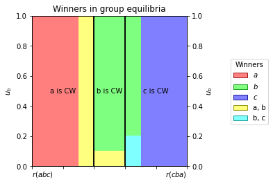
    title='Winners in group equilibria',
    legend_title='Winners',
    meth='analyzed_strategies_group')

(<Figure size 288x288 with 2 Axes>,
 <poisson_approval.meta_analysis.binary_plots.BinaryAxesSubplotPoisson at 0x1e2d24b4dd8>)

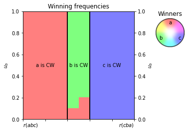
Winning Frequencies in Fictitious Play or Iterated Voting

By default, the function *binary_plot_winning_frequencies computes the winning frequencies in fictitious play, with an initialization in sincere strategy, and with all update ratios in \(1 / \log(t + 1)\):

pa.binary_plot_winning_frequencies(
    xyy_to_profile,
    xscale=XSCALE, yscale=YSCALE,
    n_max_episodes=100)

(<Figure size 288x288 with 3 Axes>,
 <poisson_approval.meta_analysis.binary_plots.BinaryAxesSubplotPoisson at 0x1e2d26dd860>)

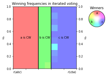
You can change this behavior with the optional parameters of the function:

pa.binary_plot_winning_frequencies(
    xyy_to_profile,
    xscale=XSCALE, yscale=YSCALE,
    meth='iterated_voting',
    init='random_tau_undominated',
    samples_per_point=10,
    perception_update_ratio=1,
    ballot_update_ratio=1,
    winning_frequency_update_ratio=pa.one_over_t,
    n_max_episodes=100,
    title='Winning frequencies in iterated voting',
    legend_title='Winners'
)

(<Figure size 288x288 with 3 Axes>,
 <poisson_approval.meta_analysis.binary_plots.BinaryAxesSubplotPoisson at 0x1e2d2973198>)

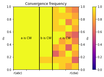
Convergence Rate in Fictitious Play or Iterated Voting

The function binary_plot_convergence computes the convergence frequency in fictitious play or iterated voting, which is defined as the proportion of initializations that lead to convergence within n_max_episodes iterations. Its syntax is similar to binary_plot_winning_frequencies.

pa.binary_plot_convergence(xyy_to_profile,
                           xscale=XSCALE, yscale=YSCALE,
                           n_max_episodes=100, init='random_tau', samples_per_point=10)

(<Figure size 414x288 with 3 Axes>,
 <poisson_approval.meta_analysis.binary_plots.BinaryAxesSubplotPoisson at 0x1e2d288de10>)

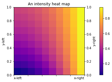
Advanced Intensity Heat Maps

First, define a function that maps a point \((x, y1, y2)\) to a number:

def f(x, y1, y2):
    return (x**2 + y1) / (y2 + 1)

Then use the method heatmap_intensity:

figure, tax = pa.binary_figure(xscale=XSCALE, yscale=YSCALE)
tax.heatmap_intensity(f,
                      x_left_label='x-left',
                      x_right_label='x-right',
                      y_left_label='y-left',
                      y_right_label='y-right')
tax.set_title('An intensity heat map')

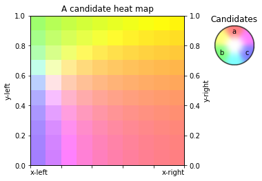
Advanced Candidate Heat Maps

First, define a function that maps a point \((x, y1, y2)\) to a list of size 3 (associated with candidates a, b, c):

def g(x, y1, y2):
    a = x**.5
    b = y1**2
    c = 1 - a - b
    return [a, b, c]

Then use the method heatmap_candidates:

figure, tax = pa.binary_figure(xscale=XSCALE, yscale=YSCALE)
tax.heatmap_candidates(g,
                       x_left_label='x-left',
                       x_right_label='x-right',
                       y_left_label='y-left',
                       y_right_label='y-right',
                       legend_title='Candidates',
                       legend_style='palette')
tax.set_title('A candidate heat map')