More Classes of Profiles

from fractions import Fraction
from matplotlib import pyplot as plt
import poisson_approval as pa

Up to now, we have always used the class of profiles ProfileNoisyDiscrete. The package provides other kinds of profiles.

ProfileHistogram

ProfileHistogram is probably the closest class to ProfileNoisyDiscrete, because both are:

• Cardinal: the voters have explicit utilities (unlike ProfileOrdinal, cf. below).

• Continuous: there is no concentration of voters on a specific utility (unlike ProfileDiscrete, cf. below).

A ProfileHistogram can be defined manually (cf. the Reference section), but it is more common to use a random factory:

rand_profile = pa.RandProfileHistogramGridUniform(
    denominator=100,
    denominator_bins=100,
    n_bins=10
)
profile = rand_profile()
profile

<abc: 3/25 [Fraction(43, 100) 0 Fraction(1, 10) Fraction(1, 25) Fraction(1, 50)
 Fraction(1, 10) Fraction(2, 25) 0 Fraction(1, 25) Fraction(19, 100)], acb: 19/50 [Fraction(3, 50) Fraction(3, 100) Fraction(7, 100) Fraction(1, 25)
 Fraction(9, 100) Fraction(2, 25) Fraction(2, 25) Fraction(1, 25)
 Fraction(12, 25) Fraction(3, 100)], bca: 3/20 [Fraction(1, 20) Fraction(1, 20) Fraction(29, 100) Fraction(17, 100)
 Fraction(3, 100) Fraction(1, 10) Fraction(1, 50) Fraction(2, 25)
 Fraction(1, 100) Fraction(1, 5)], cab: 7/100 [Fraction(1, 50) Fraction(33, 100) Fraction(13, 100) Fraction(1, 25) 0
 Fraction(17, 100) Fraction(13, 100) Fraction(3, 100) Fraction(1, 20)
 Fraction(1, 10)], cba: 7/25 [Fraction(11, 100) Fraction(3, 50) Fraction(21, 50) Fraction(3, 100)
 Fraction(9, 50) 0 Fraction(1, 10) 0 0 Fraction(1, 10)]> (Condorcet winner: a, c)

In this example, the share of voters \(abc\) is:

profile.abc

Fraction(3, 25)

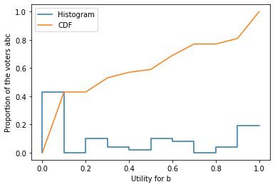
The distribution of their utility for their middle candidate \(b\) is given by a histogram:

profile.d_ranking_histogram['abc']

array([Fraction(43, 100), 0, Fraction(1, 10), Fraction(1, 25),
       Fraction(1, 50), Fraction(1, 10), Fraction(2, 25), 0,
       Fraction(1, 25), Fraction(19, 100)], dtype=object)

The above notation means for example that for a voter \(abc\), the probability that her utility for her second candidate \(b\) is in the first of the ten bins (i.e. between 0 and 0.1) is:

profile.d_ranking_histogram['abc'][0]

Fraction(43, 100)

Voters in a bin are distributed uniformly. This histogram and the CDF of this distribution can be visualized by:

ranking = 'abc'
profile.plot_histogram(ranking, label='Histogram')
profile.plot_cdf(ranking, label='CDF')
plt.ylabel('Proportion of the voters %s' % ranking)
plt.legend()

<matplotlib.legend.Legend at 0x17affbec208>

All other features are defined as usual. For example:

rand_strategy = pa.RandStrategyThresholdGridUniform(denominator_threshold=100, profile=profile)
strategy = rand_strategy()
strategy

<abc: utility-dependent (9/20), acb: utility-dependent (3/50), bca: utility-dependent (3/50), cab: utility-dependent (19/100), cba: utility-dependent (97/100)> ==> c

strategy.is_equilibrium

EquilibriumStatus.NOT_EQUILIBRIUM

ProfileTwelve

In a ProfileTwelve, the voters behave as if their utility for their middle candidate was either infinitely close to 0 or to 1. For example, voters with the ranking \(abc\) are split in two categories: voters a_bc (whose utility for \(b\) is very low) and voters ab_c (whose utility for \(b\) is very high). This can be interpreted in two ways:

• As a model of their preferences: voters a_bc have a utility for \(b\) that is very close to 1,

• As a behavioral model: when their best response is utility-dependent, voters a_bc always choose to vote \(a\) only, no matter the utility threshold of the best response.

Create a profile:

profile = pa.ProfileTwelve({'ab_c': Fraction(1, 10), 'b_ac': Fraction(6, 10),
                            'c_ab': Fraction(2, 10), 'ca_b': Fraction(1, 10)})
profile

<ab_c: 1/10, b_ac: 3/5, c_ab: 1/5, ca_b: 1/10> (Condorcet winner: b)

Share of voters ab_c:

profile.ab_c

Fraction(1, 10)

Which types are in the profile?

profile.support_in_types

{ab_c, b_ac, c_ab, ca_b}

Are all possible types in the profile?

profile.is_generic_in_types

False

Is one type shared by a majority of voters?

profile.has_majority_type

True

In addition to the usual StrategyOrdinal and StrategyThreshold, this kind of profile also accepts a StrategyTwelve:

strategy = pa.StrategyTwelve({'abc': 'ab', 'bac': 'b', 'cab': pa.UTILITY_DEPENDENT}, profile=profile)
strategy

<abc: ab, bac: b, cab: utility-dependent> ==> b

In the example above, the strategy for \(cab\) is utility-dependent, meaning that voters c_ba vote for \(c\) and voters cb_a vote for \(c\) and \(b\). One can envision it as a threshold strategy, but it is useless to specify the value of the threshold because we’re dealing with a ProfileTwelve.

profile.is_equilibrium(strategy)

EquilibriumStatus.EQUILIBRIUM

Since there is a finite number of pure strategies for a ProfileTwelve, it is possible to analyze them all:

profile.analyzed_strategies_pure

Equilibria:
<abc: a, bac: b, cab: ac> ==> b (FF)
<abc: a, bac: ab, cab: c> ==> a (D)
<abc: ab, bac: b, cab: utility-dependent> ==> b (FF)

Non-equilibria:
<abc: a, bac: b, cab: c> ==> b (FF)
<abc: a, bac: b, cab: utility-dependent> ==> b (FF)
<abc: a, bac: ab, cab: ac> ==> a (D)
<abc: a, bac: ab, cab: utility-dependent> ==> a (D)
<abc: ab, bac: b, cab: c> ==> b (FF)
<abc: ab, bac: b, cab: ac> ==> b (FF)
<abc: ab, bac: ab, cab: c> ==> a, b (FF)
<abc: ab, bac: ab, cab: ac> ==> a (D)
<abc: ab, bac: ab, cab: utility-dependent> ==> a (D)

All other features are defined as usual.

ProfileDiscrete

A ProfileDiscrete is similar to a ProfileNoisyDiscrete, but of course without noise:

profile = pa.ProfileDiscrete({
    ('abc', 0.9): Fraction(1, 10),
    ('bac', 0.2): Fraction(6, 10),
    ('cab', 0.25): Fraction(2, 10),
    ('cab', 0.75): Fraction(1, 10)
})
profile

<abc 0.9: 1/10, bac 0.2: 3/5, cab 0.25: 1/5, cab 0.75: 1/10> (Condorcet winner: b)

In the above example, the share of voters with ranking \(abc\) and a utility 0.9 for their middle candidate \(b\) is 1/10, the share of voters with ranking \(bac\) and a utility 0.2 for their middle candidate \(a\) is 3/5, etc.

The difficulty is that there is now a concentration of voters, for example, on \((abc, 0.9)\). This opens the door to mixed strategies where voters of this type split their ballots between \(a\) and \(ab\). To account for this fact, a StrategyThreshold can include ratios of optimistic voters:

strategy = pa.StrategyThreshold({
    'abc': (0.9, 0.7),
    'bac': 0.5,
    'cab': 0.5
}, profile=profile)
strategy

<abc: utility-dependent (0.9, 0.7), bac: utility-dependent (0.5), cab: utility-dependent (0.5)> ==> b

The above notation means that voters \(abc\) have:

• A utility threshold of 0.9: they vote for \(a\) (resp. \(ab\)) if their utility for their second candidate \(b\) is lower (resp. greater) than 0.9;

• An ratio of optimistic voters of 0.7: voters whose utility for \(b\) is equal to the utility threshold 0.9 are split, with 0.7 of them voting for \(a\) and the rest voting for \(ab\).

Like for ProfileTwelve, there is a finite number of pure strategies, so it is possible to analyze them all:

profile.analyzed_strategies_pure

Equilibria:
<abc: ab, bac: b, cab: utility-dependent (0.5)> ==> b (FF)
<abc: a, bac: ab, cab: c> ==> a (D)
<abc: a, bac: b, cab: ac> ==> b (FF)

Non-equilibria:
<abc: ab, bac: ab, cab: ac> ==> a (D)
<abc: ab, bac: ab, cab: utility-dependent (0.5)> ==> a (D)
<abc: ab, bac: ab, cab: c> ==> a, b (FF)
<abc: ab, bac: b, cab: ac> ==> b (FF)
<abc: ab, bac: b, cab: c> ==> b (FF)
<abc: a, bac: ab, cab: ac> ==> a (D)
<abc: a, bac: ab, cab: utility-dependent (0.5)> ==> a (D)
<abc: a, bac: b, cab: utility-dependent (0.5)> ==> b (FF)
<abc: a, bac: b, cab: c> ==> b (FF)

All other features are defined as usual.

ProfileOrdinal

A ProfileOrdinal is a bit special, in the sense that it does not represent a profile, strictly speaking, but rather a family of profiles that have the same ordinal representation.

Definition and Strategic Analysis

profile = pa.ProfileOrdinal({
    'abc': Fraction(1, 10),
    'bac': Fraction(6, 10),
    'cab': Fraction(3, 10)
})
profile

<abc: 1/10, bac: 3/5, cab: 3/10> (Condorcet winner: b)

Let us analyze its ordinal strategies:

profile.analyzed_strategies_ordinal

Equilibria:
<abc: a, bac: b, cab: ac> ==> b (FF)
<abc: a, bac: ab, cab: c> ==> a (D)

Utility-dependent equilibrium:
<abc: ab, bac: b, cab: c> ==> b (FF)

Non-equilibria:
<abc: a, bac: b, cab: c> ==> b (FF)
<abc: a, bac: ab, cab: ac> ==> a (D)
<abc: ab, bac: b, cab: ac> ==> b (FF)
<abc: ab, bac: ab, cab: c> ==> a, b (FF)
<abc: ab, bac: ab, cab: ac> ==> a (D)

In the example above, there are not only equilibria and non-equilibria but also a new category of strategies: utility-dependent equilibria. For example:

strategy = profile.analyzed_strategies_ordinal.utility_dependent[0]
strategy

<abc: ab, bac: b, cab: c> ==> b

strategy.d_ranking_best_response['abc']

<ballot = ab, utility_threshold = 0, justification = Asymptotic method>

strategy.d_ranking_best_response['bac']

<ballot = utility-dependent, utility_threshold = 0.836014, justification = Asymptotic method>

strategy.d_ranking_best_response['cab']

<ballot = utility-dependent, utility_threshold = 0.163986, justification = Asymptotic method>

What happens here? For example, the best response for voters \(bac\) is utility-dependent, with a utility threshold of 0.84 approximately. The fact that they vote \(b\) in strategy is indeed a best response if and only if their utility for their second candidate \(a\) is lower than this value. Overall, strategy is an equilibrium if and only if:

• The utility of voters \(bac\) for \(a\) is lower than 0.84,

• And the utility of voters \(cab\) for \(a\) is lower than 0.16.

Probability computations

The following functions compute probabilities. They are based on the assumption that voters \(abc\) have the same utility for their second candidate \(b\) and that it is drawn uniformly in [0, 1]. And similarly for voters \(acb\), \(bac\), etc.

Probability that there exists an equilibrium:

profile.proba_equilibrium()

1

In this example, the probability is 1 because there exists some equilibria that do not depend on the utilities.

Probability that there exists an equilibrium where voters \(abc\) cast a ballot \(ab\):

def test_abc_vote_ab(strategy):
    return strategy.abc == 'ab'
profile.proba_equilibrium(test=test_abc_vote_ab)

0.13709468816628012

Probability that there exists an equilibrium where candidate \(c\) wins:

def test_c_wins(strategy):
    return 'c' in strategy.winners
profile.proba_equilibrium(test=test_c_wins)

0

Distribution of the number of equilibria:

profile.distribution_equilibria()

array([0.        , 0.        , 0.86290531, 0.13709469])

The above array means that it is impossible that there is 0 or 1 equilibrium, a probability 0.86 to have 2 equilibria, and a probability 0.14 to have 3 equilibria.

You can access the distribution of equilibria, conditionally on a given test:

profile.distribution_equilibria(test=test_abc_vote_ab)

array([0.86290531, 0.13709469])

The above array means that there is a probability 0.86 to have no equilibrium, and a probability 0.14 to have one equilibrium (conditionally on the given test).

Distribution of the number of winners at equilibrium:

profile.distribution_winners()

array([0, 0, 1, 0])

The array above means that there are always 2 candidates (namely \(a\) and \(b\)) who can win at equilibrium.

You can access the distribution of winners, conditionally on a given test:

profile.distribution_winners(test=test_abc_vote_ab)

array([0.86290531, 0.13709469, 0.        , 0.        ])

The above array means that there is a probability 0.86 of having 0 winner (i.e. when there is no equilibrium), and a probability 0.14 to have 1 winner (conditionally on the given test).