Probabilities
[1]:
from matplotlib import pyplot as plt
from fractions import Fraction
import poisson_approval as pa
Random Factories
The package provides a large variety of random factories to generate profiles, strategies or tau-vectors. For example, define a random factory of tau-vectors:
[2]:
rand_tau = pa.RandTauVectorUniform()
Then use this random factory to generate a tau-vector:
[3]:
tau = rand_tau()
tau
[3]:
<a: 0.01026179823073825, ab: 0.15335471082695618, ac: 0.18428374829679528, b: 0.10894428401103218, bc: 0.535560376132927, c: 0.007595082501551165> ==> b
Most random factories of the package also have a “grid” counterpart where the coefficients are fractions of a given denominator. This is convenient to generate less “messy” examples:
[4]:
rand_tau = pa.RandTauVectorGridUniform(denominator=100)
tau = rand_tau()
tau
[4]:
<a: 1/4, ab: 2/25, ac: 1/100, b: 1/20, bc: 19/50, c: 23/100> ==> c
Also, most random factories have options that enable to finely tune the distribution:
[5]:
rand_tau = pa.RandTauVectorUniform(
    ballots=['a', 'b'],
    d_ballot_fixed_share={'c': 0.1},
    voting_rule=pa.PLURALITY
)
tau = rand_tau()
tau
[5]:
<a: 0.7678442160616922, b: 0.13215578393830785, c: 0.1> ==> a (Plurality)
For more information, cf. the Reference section on random factories.
Conditional Random Factory
RandConditional is a random factory implementing rejection sampling. It needs:
Another random factory that is responsible for generating the objects,
A test that the objects must meet,
A maximum number of trials before renouncing (which can be None if you want to draw objects forever, until finding one that meets the test).
Here, we use a conditional random factory to generate an example of TauVector with a direct focus:
[6]:
def test_direct_focus(tau):
    return tau.focus == pa.Focus.DIRECT
[7]:
rand_tau = pa.RandConditional(
    factory=pa.RandTauVectorGridUniform(denominator=100),
    test=test_direct_focus,
    n_trials_max=None
)
tau = rand_tau()
tau
[7]:
<a: 19/100, ab: 8/25, ac: 1/100, b: 19/100, bc: 17/100, c: 3/25> ==> b
Alternatively, RandConditional accepts a tuple of factories, and a test on the tuple of the results. Here is an example of a ProfileNoisyDiscrete and a StrategyOrdinal, such that the strategy is an equilibrium for the profile:
[8]:
rand_profile = pa.RandProfileNoisyDiscreteGridUniform(
    denominator=100,
    types=[('abc', 0.4, 0.01),
           ('bac', 0.2, 0.01),
           ('cab', 0.7, 0.01)]
)
rand_strategy = pa.RandStrategyOrdinalUniform()
def test_is_equilibrium(profile, strategy):
    return profile.is_equilibrium(strategy) == pa.EquilibriumStatus.EQUILIBRIUM
[9]:
rand_example = pa.RandConditional(
    factory=(rand_profile, rand_strategy),
    test=test_is_equilibrium,
    n_trials_max=None
)
profile, strategy = rand_example()
print(profile)
print(strategy)
<abc 0.4 ± 0.01: 9/20, bac 0.2 ± 0.01: 41/100, cab 0.7 ± 0.01: 7/50> (Condorcet winner: a)
<abc: a, acb: a, bac: ab, bca: bc, cab: c, cba: c>
Probability Estimation
To compute a probability, use the function probability.
For example, estimate the probability that a TauVector drawn uniformly at random has a direct focus:
[10]:
def test_direct_focus(tau):
    return tau.focus == pa.Focus.DIRECT
[11]:
pa.probability(
    factory=pa.RandTauVectorUniform(),
    n_samples=100,
    test=test_direct_focus
)
[11]:
0.43
To avoid the definition of an auxiliary function, you can use a lambda. For example:
[12]:
pa.probability(
    factory=pa.RandTauVectorUniform(),
    n_samples=100,
    test=lambda tau: tau.focus == pa.Focus.DIRECT
)
[12]:
0.52
You can also compute a conditional probability. For example, the probability that a ProfileNoisyDiscrete (generated by the random factory defined below) has an ordinal equilibrium, conditionally on having a strict Condorcet winner:
[13]:
rand_profile = pa.RandProfileNoisyDiscreteUniform(
    types=[('abc', 0.4, 0.01),
           ('bac', 0.2, 0.01),
           ('cab', 0.7, 0.01)]
)
def test_exists_ordinal_equilibrium(profile):
    return len(profile.analyzed_strategies_ordinal.equilibria) > 0
def test_is_strictly_condorcet(profile):
    return profile.is_profile_condorcet == 1.0
[14]:
pa.probability(
    factory=rand_profile,
    n_samples=100,
    test=test_exists_ordinal_equilibrium,
    conditional_on=test_is_strictly_condorcet
)
[14]:
1.0
You can also use a tuple of random factories, and tests on the tuple of the results. For example, estimate the probability that a random StrategyOrdinal is an equilibrium for a random ProfileNoisyDiscrete (generated by the random factory defined below), conditionally on the fact that the profile has a strict Condorcet winner and that the initial strategy elects the Condorcet winner:
[15]:
rand_profile = pa.RandProfileNoisyDiscreteUniform(
    types=[('abc', 0.4, 0.01),
           ('bac', 0.2, 0.01),
           ('cab', 0.7, 0.01)]
)
rand_strategy = pa.RandStrategyOrdinalUniform()
def test_is_equilibrium(profile, strategy):
    return profile.is_equilibrium(strategy) == pa.EquilibriumStatus.EQUILIBRIUM
def test_elect_condorcet_winner(profile, strategy):
    return (profile.is_profile_condorcet == 1.
            and profile.tau(strategy).winners == profile.condorcet_winners)
[16]:
pa.probability(
    factory=(rand_profile, rand_strategy),
    n_samples=100,
    test=test_is_equilibrium,
    conditional_on=test_elect_condorcet_winner
)
[16]:
0.36
Finally, you can also use a tuple of tests in order to estimate several probabilities with the same sample. For example, estimate the probability that a TauVector drawn uniformly at random is direct, forward-focused, backward-focused, or unfocused:
[17]:
pa.probability(
    factory=pa.RandTauVectorUniform(),
    n_samples=100,
    test=(lambda tau: tau.focus == pa.Focus.DIRECT,
          lambda tau: tau.focus == pa.Focus.FORWARD_FOCUSED,
          lambda tau: tau.focus == pa.Focus.BACKWARD_FOCUSED,
          lambda tau: tau.focus == pa.Focus.UNFOCUSED)
)
[17]:
(0.52, 0.48, 0.0, 0.0)
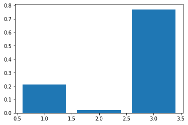
Image Distribution Estimation
To compute an image distribution, use the function image_distribution.
For example, when drawing a ProfileNoisyDiscrete (with the random factory defined below) and an initial StrategyOrdinal at random, and when applying iterated voting, let us estimate the distribution of the length of the cycle to which it converges:
[18]:
rand_profile = pa.RandProfileNoisyDiscreteUniform(
    types=[('abc', 0.4, 0.01),
           ('bca', 0.2, 0.01),
           ('cab', 0.7, 0.01)]
)
rand_strategy = pa.RandStrategyOrdinalUniform()
[19]:
def len_cycle(profile, strategy_ini):
    cycle = profile.iterated_voting(init=strategy_ini, n_max_episodes=100)['cycle_taus_actual']
    return len(cycle)
[20]:
d_len_occurrences = pa.image_distribution(
    factory=(rand_profile, rand_strategy),
    n_samples=100, f=len_cycle)
d_len_occurrences
[20]:
{1: 0.21, 2: 0.02, 3: 0.77}
[21]:
plt.bar(d_len_occurrences.keys(), d_len_occurrences.values())
[21]:
<BarContainer object of 3 artists>