Monte-Carlo Fictitious Play

[1]:

import poisson_approval as pa

The goal of Monte-Carlo fictitious play is to perform fictitious play on several profiles drawn at random. First, define a random factory of profiles:

[2]:

rand_profile= pa.RandProfileNoisyDiscreteUniform(
    types=[(ranking, 0.5) for ranking in pa.RANKINGS],
    noise=0.5
)

Here, we consider profiles of the class ProfileNoisyDiscreteUniform, and we specify that the possible types are all rankings, with a utility 0.5 for their middle candidate, and with a noise of 0.5: in other words, their utility for their middle candidate is uniformly drawn on the interval (0, 1).

Launch Monte-Carlo fictitious play:

[3]:

meta_results = pa.monte_carlo_fictitious_play(
    factory=rand_profile,
    n_samples=100,
    n_max_episodes=100,
    voting_rules=pa.VOTING_RULES,
    init='random_tau',
    monte_carlo_settings=[
        pa.MCS_BALLOT_STATISTICS,
        pa.MCS_CANDIDATE_WINNING_FREQUENCY,
        pa.MCS_CONVERGES,
        pa.MCS_DECREASING_SCORES,
        pa.MCS_N_EPISODES,
        pa.MCS_PROFILE,
        pa.MCS_TAU_INIT,
        pa.MCS_UTILITY_THRESHOLDS,
        pa.MCS_WELFARE_LOSSES
    ],
)

According to the options we entered, we use the factory rand_profile defined above, we draw n_samples=100 profiles, fictitious play is performed with a maximum of n_max_episodes=100 episodes, for all the voting rules of the package (Approval, Plurality, Anti-Plurality). For each profile, fictitious play is initialized with the option 'random_tau', i.e. with a tau-vector drawn uniformly at random. The list monte_carlo_settings gives some additional options: each of them provides a “bundle” of statistics that will be computed during the process. For example, the option MCS_CONVERGES gives access to the two statistics 'converges' and 'mean_converges'. Let us see their results for Approval.

[4]:

print(meta_results[pa.APPROVAL]['converges'])

[False, True, True, True, True, True, False, True, True, True, True, True, True, True, True, True, True, True, True, True, True, True, True, True, True, True, True, True, True, True, True, True, True, True, True, True, True, True, True, True, True, True, True, True, True, True, True, True, True, True, True, True, True, True, True, True, True, True, True, True, True, True, True, True, True, True, True, True, True, True, True, True, True, True, True, True, True, True, True, True, True, True, True, True, True, True, True, True, True, True, True, True, True, True, False, True, True, True, False, True]

For each profile drawn, the above list indicates whether fictitious play has converged or not.

[5]:

print(meta_results[pa.APPROVAL]['mean_converges'])

0.96

The above number is the rate of convergence (over all profiles).

Plot the distribution (CDF) of scores for the winner, the challenger and the loser (here for Approval):

[6]:

pa.plot_distribution_scores(
    meta_results,
    voting_rule=pa.APPROVAL
)

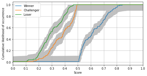
../_images/tutorials_tutorial_monte_carlo_fictitious_play_13_0.png

The gray areas represent 95% confidence intervals.

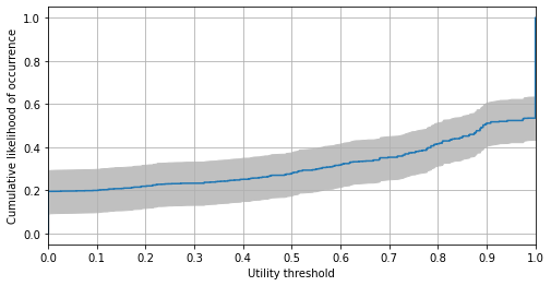
Plot the distribution (CDF) of the utility threshold (here for Approval):

[7]:

pa.plot_utility_thresholds(
    meta_results,
    voting_rule=pa.APPROVAL
)

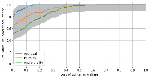
../_images/tutorials_tutorial_monte_carlo_fictitious_play_16_0.png

Plot the distribution (CDF) of the welfare loss (for all voting rules):

[8]:

pa.plot_welfare_losses(
    meta_results,
    criterion='utilitarian_welfare_losses'
)

../_images/tutorials_tutorial_monte_carlo_fictitious_play_18_0.png

For more information, cf. the Reference section on Monte-Carlo fictitious play.