Ternary Plots

import poisson_approval as pa
from fractions import Fraction

SimplexToProfile

Poisson Approval relies on the package python-ternary to draw plots on the simplex of \(\mathbb{R}^3\). The coordinates of a point are denoted right, top and left because they are respectively equal to 1 at the right, top and left corners of the triangular figure. They typically represent shares of different types in a profile. In order to draw plots, we need a SimplexToProfile object that will generate the needed profiles:

simplex_to_profile = pa.SimplexToProfile(
    pa.ProfileNoisyDiscrete,
    right_type='c>a~b',
    top_type=('abc', 0.5, 0.01),
    left_type=('bac', 0.5, 0.01),
    d_type_fixed_share={('abc', 0.1, 0.01): Fraction(1, 10),
                        ('abc', 0.9, 0.01): Fraction(1, 10)}
)

The above syntax defines a function simplex_to_profile that maps a tuple (right, top, left) to a profile defined as:

• The class of profile is ProfileNoisyDiscrete,

• A fixed share 1/10 of voters are of type \((abc, 0.1, 0.01)\), and a fixed share 1/10 of voters are of type \((abc, 0.9, 0.01)\),

• The other voters, i.e. a share 8/10, are distributed between right_type, top_type and left_type, in respective proportions that are given by the input tuple (right, top, left).

For example:

simplex_to_profile(right=Fraction(17, 80), top=Fraction(52, 80), left=Fraction(11, 80))

<abc 0.1 ± 0.01: 1/10, abc 0.5 ± 0.01: 13/25, abc 0.9 ± 0.01: 1/10, bac 0.5 ± 0.01: 11/100, c>a~b: 17/100> (Condorcet winner: a)

Scale

All the plots require a resolution parameter called scale. For example, if scale=10, then the simplex is divided into cells of diameter 1/10 and the value of the plotted function is computed at the center of each cell. For more information, cf. the documentation of the package python-ternary. In this tutorial, we define a global parameter SCALE and we will use it for all the plots.

SCALE = 21

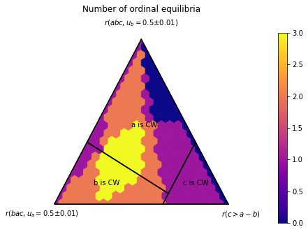
Number of Equilibria

By default, the function ternary_plot_n_equilibria computes the ordinal equilibria, i.e. those where all voters having the same ranking cast the same ballot:

pa.ternary_plot_n_equilibria(
    simplex_to_profile,
    scale=SCALE,
    title='Number of ordinal equilibria')

(<Figure size 504x360 with 2 Axes>, TernaryAxesSubplot: -9223371904852674332)

Using the option meth, you can investigate other kinds of equilibria:

pa.ternary_plot_n_equilibria(
    simplex_to_profile,
    scale=SCALE,
    title='Number of group equilibria',
    meth='analyzed_strategies_group')

(<Figure size 504x360 with 2 Axes>, TernaryAxesSubplot: 132002423279)

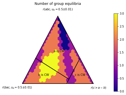
Depending on the class of profile, the possible values of the option meth may be:

• 'analyzed_strategies_ordinal' (the default),

• 'analyzed_strategies_group' (for profiles where a reasonable notion of group is defined, such as ProfileNoisyDiscrete),

• 'analyzed_strategies_pure' (for discrete profiles such as ProfileDiscrete or ProfileTwelve).

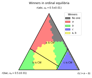
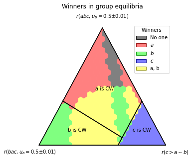
Winners at Equilibrium

The function ternary_plot_n_equilibria works similarly:

pa.ternary_plot_winners_at_equilibrium(
    simplex_to_profile,
    scale=SCALE,
    title='Winners in ordinal equilibria')

(<Figure size 360x360 with 1 Axes>, TernaryAxesSubplot: -9223371904852273148)

pa.ternary_plot_winners_at_equilibrium(
    simplex_to_profile,
    scale=SCALE,
    title='Winners in group equilibria',
    legend_title='Winners',
    meth='analyzed_strategies_group')

(<Figure size 360x360 with 1 Axes>, TernaryAxesSubplot: -9223371904852057000)

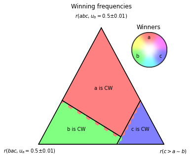
Winning Frequencies in Fictitious Play or Iterated Voting

By default, the function ternary_plot_winning_frequencies computes the winning frequencies in fictitious play, with an initialization in sincere strategy, and with all update ratios in \(1 / \log(t + 1)\):

pa.ternary_plot_winning_frequencies(simplex_to_profile, scale=SCALE, n_max_episodes=100)

(<Figure size 360x360 with 2 Axes>, TernaryAxesSubplot: 132002943727)

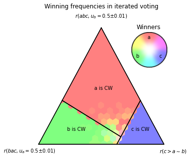
You can change this behavior with the optional parameters of the function:

pa.ternary_plot_winning_frequencies(
    simplex_to_profile,
    scale=SCALE,
    meth='iterated_voting',
    init='random_tau_undominated',
    samples_per_point=10,
    perception_update_ratio=1,
    ballot_update_ratio=1,
    winning_frequency_update_ratio=pa.one_over_t,
    n_max_episodes=100,
    title='Winning frequencies in iterated voting',
    legend_title='Winners'
)

(<Figure size 360x360 with 2 Axes>, TernaryAxesSubplot: -9223371904850416903)

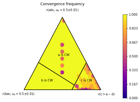
Convergence Rate in Fictitious Play or Iterated Voting

The function ternary_plot_convergence computes the convergence frequency in fictitious play or iterated voting, which is defined as the proportion of initializations that lead to convergence within n_max_episodes iterations. Its syntax is similar to ternary_plot_winning_frequencies.

pa.ternary_plot_convergence(simplex_to_profile, scale=SCALE, n_max_episodes=100,
                            init='random_tau', samples_per_point=10)

(<Figure size 504x360 with 2 Axes>, TernaryAxesSubplot: 132005039936)

Customize the Plot

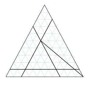
Grid and lines:

figure, tax = pa.ternary_figure()
tax.gridlines_simplex(multiple=0.1)
tax.horizontal_line_simplex(0.1)
tax.left_parallel_line_simplex(0.2)
tax.right_parallel_line_simplex(0.3)
tax.line_simplex((1, 0, 0), (0.2, 0.5, 0.3))

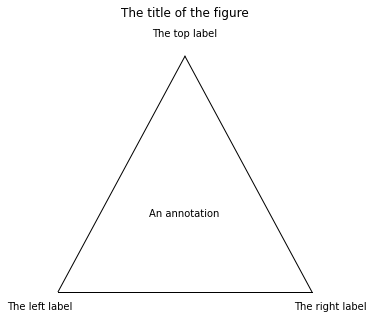
Titles and annotations:

figure, tax = pa.ternary_figure()
tax.set_title_padded('The title of the figure')
tax.right_corner_label('The right label')
tax.top_corner_label('The top label')
tax.left_corner_label('The left label')
tax.annotate_simplex('An annotation', (0.33, 0.33, 0.33))

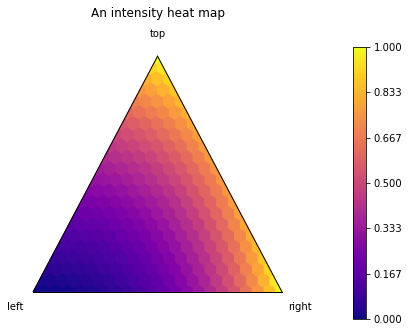
Advanced Intensity Heat Maps

First, define a function that maps a point of the simplex to a number:

def f(right, top, left):
    return (right**2 + top) / (left + 1)

Then use the method heatmap_intensity:

figure, tax = pa.ternary_figure(scale=SCALE)
tax.heatmap_intensity(f,
                      left_label='left',
                      right_label='right',
                      top_label='top')
tax.set_title_padded('An intensity heat map')

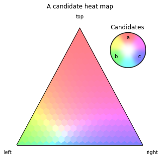
Advanced Candidate Heat Maps

First, define a function that maps a point of the simplex to a list of size 3 (associated with candidates a, b, c):

def g(right, top, left):
    a = top**.5
    b = left**2
    c = 1 - a - b
    return [a, b, c]

Then use the method heatmap_candidates:

figure, tax = pa.ternary_figure(scale=SCALE)
tax.heatmap_candidates(g,
                       left_label='left',
                       right_label='right',
                       top_label='top',
                       legend_title='Candidates',
                       legend_style='palette')
tax.set_title_padded('A candidate heat map')